


We last left off studying the heat equation in the one-dimensional case of a rod the question is how the temperature distribution along such a rod will tend to change over time and This gave us a nice first example for a partial differential equation It told us that the rate at which the temperature at a given point changes over time Depends on the second derivative of that temperature at that point with respect to space where there's curvature in space there's change in time Here we're gonna look at how to solve that equation And actually it's a little misleading to refer to all of this as solving an equation The PDE itself only describes one out of three constraints that our temperature function must satisfy If it's gonna accurately describe heat flow, it must also satisfy certain boundary conditions Which is something we'll talk about momentarily and a certain initial condition That is you don't get to choose how it looks at time T equals zero that's part of the problem statement These added constraints are really where all of the challenge actually lies there is a vast ocean of function solving the PDE in the sense that when you take their partial derivatives the thing is going to Be equal and a sizable subset of that ocean satisfies the right boundary conditions When Joseph Fourier solved this problem in 1822 his key contribution was to gain control of this ocean Turning all of the right knobs and dials.
So as to be able to select from it the particular solution fitting a given initial condition We can think of his solution as being broken down into three fundamental observations Number one certain sine waves offer a really simple solution to this equation number two If you know multiple solutions the sum of these functions is also a solution and number three most surprisingly any Function can be expressed as a sum of sine waves Well a pedantic mathematician might point out that there are some pathological exceptions certain weird functions where this isn't true But basically any distribution that you would come across in practice including discontinuous ones can be written as a sum of sine waves potentially infinitely many and if you've ever heard of Fourier series, you've at least heard of this last idea and if so, Maybe you've wondered why on earth. Would anyone care about breaking down a function as some of sine waves Well in many applications sine waves are nicer to deal with than anything else and differential equations offers us a really nice context Where you can see how that plays out for our heat equation when you write a function as a sum of these waves the relatively clean second derivatives makes it easy to solve the heat equation for each one of them and As you'll see a sum of solutions to this equation Gives us another solution and so in turn that will give us a recipe for solving the heat equation for any complicated distribution as an initial state here Let's dig into that first step why exactly would sign waves play nicely with the heat equation to avoid messy constants let's start simple and say that the temperature function at time T equals zero is Simply sine of X where X describes the point on the rod Yes, the idea of a-rod's temperature Just happening to look like sine of X varying around whatever temperature our conventions arbitrarily label a zero is clearly absurd but in math You should always be happy to play with examples that are idealized potentially Well beyond the point of being realistic because they can offer a good first step in the direction of something more general and hence more realistic The right-hand side of this heat equation asks about the second derivative of our function How much our temperature distribution curves as you move along space? The derivative of sine of X is cosine of X Whose derivative in turn is negative sine of X the amount that wave curves is in a sense Equal and opposite to its height at each point So at least at the time T equals zero This has the peculiar effect that each point changes its temperature at a rate proportional to the temperature of the point itself with the same proportionality constant across all points So after some tiny time step everything scales down by the same factor and after that It's still the same sine curve shape just scale down a bit So the same logic applies and the next time step would scale it down Uniformly again and this applies just as well in the limit as the size of these time steps approaches zero So unlike other temperature distributions sine waves are peculiar in that they'll get scaled down uniformly Looking like some constant times sine of X for all times T Now when you see that the rate at which some value changes is proportional to that value itself your mind should burn with the thought of an exponential and if it's not or if you're a little rusty on the idea of taking Derivatives of Exponential's or what makes the number e special I'd recommend you take a look at this video the upshot is that the derivative of e to some constant times T is equal to that constant times itself if the rate at which your investment grows for example is always say 0.05 times the total value then its value over time is going to look like e to the 0.05 times T times whatever the initial investment was if The rate at which the count of carbon-14 atoms and an old bone changes is always equal to some negative Constant times that count itself then over time that number will look approximately like e to that negative constant times T times whatever the initial count was So when you look at our heat equation and you know that for a sine wave the right-hand side is going to be negative alpha times the temperature function itself Hopefully it wouldn't be too surprising to propose that the solution is to scale down by a factor of e to the negative alpha T Here go ahead and check the partial derivatives the proposed function of X and T is sine of X times e to the negative alpha T Taking the second partial derivative with respect to X that e to the negative alpha T term looks like a constant It doesn't have any X in it So it just comes along for the ride as if it was any other Constant like 2 and the first derivative with respect to X is cosine of X times e to the negative alpha T likewise the second partial derivative with respect to X becomes negative sine of X times e to the negative alpha T and on the flip side If you look at the partial derivative with respect to T That sine of X term now looks like a constant since it doesn't have a T in it So we get negative alpha times e to the negative alpha T times sine of X so indeed This function does make the partial differential equation true And oh, if it was only that simple this narrative flow could be so nice We would just beeline directly to the delicious Fourier series conclusion sadly nature is not so nice knocking us off onto an annoying But highly necessary detour Here's the thing even if nature were to somehow produce a temperature distribution on this rod Which looks like this perfect sine wave the exponential decay is not actually how it would evolve Assuming that no heat flows in or out of the rod Here's what that evolution would actually look like the points on the left are heated up a little at first and those on the right are cooled down by their neighbors to the interior in Fact let me give you an even simpler solution to the PDE which fails to describe actual heat flow a straight line That is the temperature function will be some nonzero constant times X and never change over time The second partial derivative with respect to X is indeed zero I mean there is no curvature and it's partial derivative with respect to time is also zero since it never changes over time And yet if I throw this into the simulator, it does actually change over time slowly approaching a uniform temperature at the mean value What's going on here? Is that the simulation I'm using treats the two boundary points of the rod Differently from how it treats all the others Which is a more accurate reflection of what would actually happen in nature if you'll recall from the last video the intuition for where that second derivative with respect to X actually came from Was rooted in having each point tend towards the average value of its two neighbors on either side But at the boundary there is no neighbor to one side If we went back to thinking of the discrete version modeling only finitely many points on this rod you could have each boundary point simply tend towards its one neighbor at a rate proportional to their difference as We do this for higher and higher resolutions notice how pretty much immediately after the clock starts Our distribution looks flat at either of those two boundary points In fact in the limiting case as these finer and finer Discretized setups approach a continuous curve the slope of our curve at the boundary will be zero for all times after the start One way this is often described.
Is that the slope at any given point is proportional to the rate of heat flow at that point? so if you want to model the restriction that no heat flows into or out of the rod the Slope at either end will be zero That's somewhat hand wavy and incomplete I know so if you want the fuller details, I've left links and resources in the description Taking the example of a straight line whose slope at the boundary points is decidedly not Zero as soon as the clock starts those boundary values will shift in Phantasmal II such that the slope there suddenly becomes zero and remains that way through the remainder of the evolution in other words Finding a function satisfying the heat equation itself is not enough It must also satisfy the property that it's flat at each of those end points for all x greater than zero phrased more precisely the partial derivative with respect to X of our temperature function at Zero T and at LT must be zero for all times T greater than zero where L is the length of the rod This is an example of a boundary condition and pretty much any time that you have to solve a partial differential equation in practice there Will also be some boundary condition hanging along for the ride which demands just as much attention as the PDE itself all of this may make it feel like we've gotten nowhere but the function which is a sine wave in space and an Exponential decay in time actually gets us quite close We just need to tweak it a little bit so that it's flat at both end points First off notice that we could just as well use a cosine function instead of a sine.

I mean, it's the same wave It's just shifted and phased by a quarter of the period which would make it flat at x equals zero as we want The second derivative of cosine of X is also negative 1 times itself So for all the same reasons as before the product cosine of x times e to the negative alpha T still satisfies the PDE To make sure that it also satisfies the boundary condition on that right side. We're going to adjust the frequency of the wave however That will affect the second derivative since higher frequency waves curve more sharply and lower frequency one's curve more gently Changing the frequency means introducing some constant. Say Omega Multiplied by the input of this function a higher value of Omega means the wave oscillates more quickly Since as you increase X the input to the cosine increases more rapidly Taking the derivative with respect to X we still get negative sign but the chain rule tells us to multiply that Omega on the outside and Similarly, the second derivative will still be negative cosine but now with Omega squared this means that the right-hand side of our equation has now picked up this Omega squared term, so To balance things out on the left-hand side.
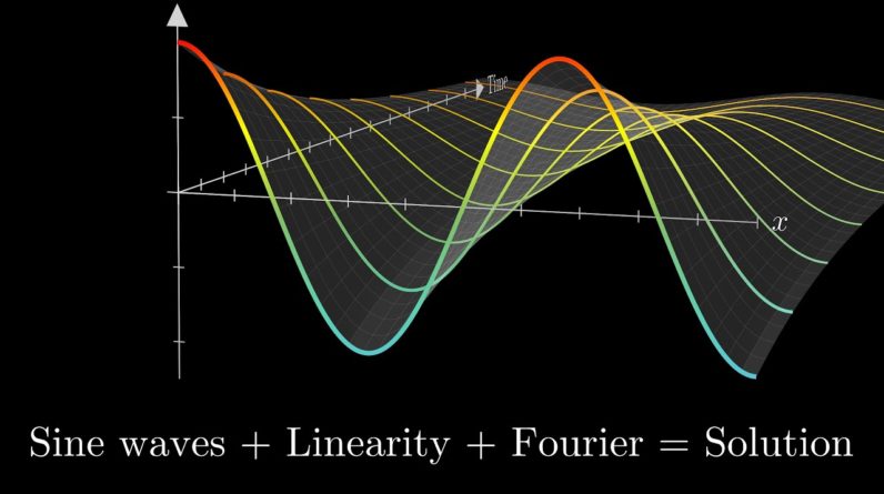
The exponential decay part should have an additional Omega squared term up top Unpacking what that actually means should feel intuitive for a temperature function filled with sharper curves It decays more quickly towards an equilibrium and evidently it Does this quadratically for instance doubling the frequency results in an exponential decay four times as fast? If the length of the rod is L Then the lowest frequency where that rightmost point of the distribution will be flat is when Omega is equal to PI divided by L See that way as x increases up to the value L The input of our cosine expression goes up to PI, which is half the period of a cosine wave Finding all the other frequencies which satisfy this boundary condition is sort of like finding harmonics You essentially go through all the whole number multiples of this base frequency PI over L In fact Even multiplying it by zero works since that gives us a constant function which is indeed a valid solution Boundary condition in all and with that we're off the bumpy boundary condition detour and back onto the freeway Moving forward were equipped with an infinite family of functions satisfying both the PDE and the pesky boundary condition Things are definitely looking more intricate now but it all stems from the one basic observation that a function which looks like a sine curve in space and an exponential decay in time fits this equation relating second derivatives in space with first derivatives in time and Of course your formulas should start to look more intricate.
You're solving a genuinely hard problem This actually makes for a pretty good stopping point So let's call it an end here and in the next video we'll look at how to use this infinite family to construct a more general solution to any of you worried about dwelling too much on a single example in a series that's meant to give a general overview of differential equations It's worth emphasizing that many of the considerations which pop up here are frequent themes throughout the field First off the fact that we modeled the boundary with its own special rule while the main differential equation only Characterized the interior is a very regular theme and a pattern well worth getting used to especially in the context of PDEs Also take note of how what we're doing is breaking down a general situation into simpler idealized cases this strategy comes up all the time and it's actually quite common for these simpler cases to look like some mixture of sine curves and Exponential's that's not at all unique to the heat equation And as time goes on we're going to get a deeper feel for why that's true